Basic Concepts
- When evaluating a classification model, predictions are compared with the actual (ground truth) labels.
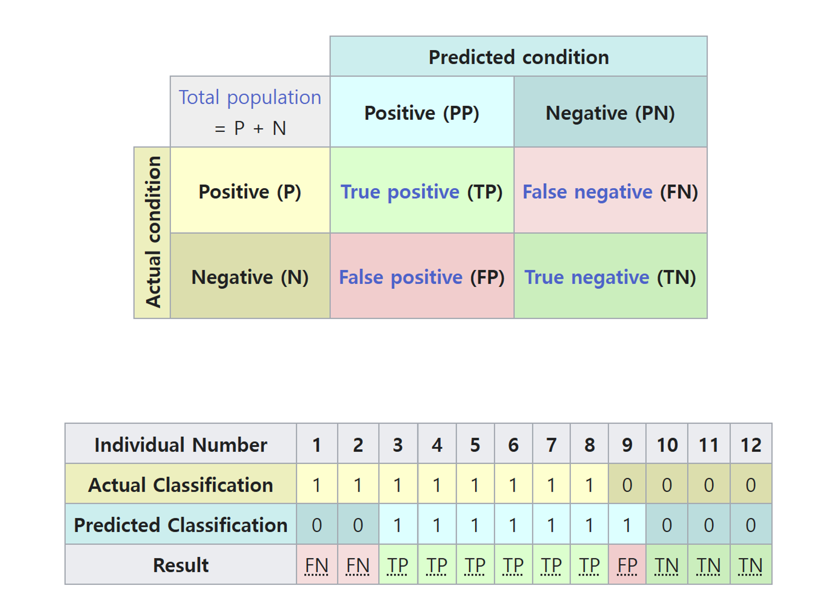
True Positive (TP)
- The model correctly predicts the positive class.
- Actual: 1 (positive).
- Predicted: 1 (positive).
False Positive (FP) (Type I Error)
- The model predicts the positive class, but the actual class is negative.
- Actual: 0 (negative).
- Predicted: 1 (positive).
- In disease detection, marking a normal person as patient.
True Negative (TN)
- The model correctly predicts the negative class.
- Actual: 0 (negative).
- Predicted: 0 (negative).
- Indicates how well the model identifies the negative class.
False Negative (FN) (Type II Error)
- The model predicts the negative class, but the actual class is positive.
- Actual: 1 (positive).
- Predicted: 0 (negative).
- In disease detection, failing to identify a patient with the disease.
Confusion matrix from wiki
Accuracy
- Accuracy is one of the most straightforward and commonly used metrics to evaluate the performance of a classification model.
- It measures the proportion of correctly classified samples out of the total number of samples.
\[
\text{Accuracy} = \frac{\text{Number of Correct Predictions}}{\text{Total Number of Predictions}}
\]
- In terms of the confusion matrix, accuracy can also be expressed as:
\[
\text{Accuracy} = \frac{\text{True Positives (TP)} + \text{True Negatives (TN)}}{\text{Total Number of Samples (TP + TN + FP + FN)}}
\]
- Good
- When the dataset is balanced, meaning the number of positive and negative samples is roughly equal.
- When all misclassification errors (false positives and false negatives) are equally costly.
- Easy to understand and implement.
- Works well for balanced datasets.
- No good
- when the dataset is imbalanced:
- For example, if 95% of the samples belong to 1, a model that always predicts the majority class will achieve 95% accuracy, but this is misleading.
- Accuracy treats all errors equally, which is not suitable if false positives and false negatives have different costs.
from sklearn.metrics import accuracy_score

# Ground truth labels and model predictions
y_true = [1, 0, 1, 1, 0, 1, 0, 0, 1, 0]
y_pred = [1, 0, 1, 0, 0, 1, 0, 0, 1, 1]

TP = sum(1 for yt, yp in zip(y_true, y_pred) if yt == 1 and yp == 1)
TN = sum(1 for yt, yp in zip(y_true, y_pred) if yt == 0 and yp == 0)
FP = sum(1 for yt, yp in zip(y_true, y_pred) if yt == 0 and yp == 1)
FN = sum(1 for yt, yp in zip(y_true, y_pred) if yt == 1 and yp == 0)
accuracy = (TP + TN) / (TP + TN + FP + FN)
print(f"Accuracy: {accuracy * 100:.2f}%")

accuracy = accuracy_score(y_true, y_pred)
print(f"Accuracy: {accuracy * 100:.2f}%")
Accuracy: 80.00%
Accuracy: 80.00%
Precision
- Of all the samples predicted as positive, how many are truly positive?
- It measures the proportion of true positive predictions out of all the samples that were predicted as positive.
\[
\text{Precision} = \frac{\text{True Positives (TP)}}{\text{True Positives (TP)} + \text{False Positives (FP)}}
\]
Precision is critical in scenarios where incorrectly predicting positives (FP) has significant consequences.
High precision ensures the model is not making too many false positive predictions, thus reducing “false alarms.”
Good
- Ensures positive predictions are reliable.
- Helps reduce “false alarms” in critical systems.
- Precision is especially useful for imbalanced datasets where the positive class is rare.
No Good
- Precision does not account for cases where the model misses actual positives (FN).
- In situations where identifying all positives is crucial (e.g., disease detection), precision alone is insufficient.
from sklearn.metrics import precision_score

# True labels
y_true = [1, 0, 1, 1, 0, 1, 0, 0, 1, 0]

# Predicted labels
y_pred = [1, 0, 1, 0, 0, 1, 0, 0, 1, 1]

TP = sum(1 for yt, yp in zip(y_true, y_pred) if yt == 1 and yp == 1)
FP = sum(1 for yt, yp in zip(y_true, y_pred) if yt == 0 and yp == 1)
precision = TP / (TP + FP)
print(f"Precision: {precision * 100:.2f}%")

# Compute precision
precision = precision_score(y_true, y_pred)
print(f"Precision: {precision * 100:.2f}%")
Precision: 80.00%
Precision: 80.00%
Recall
- Of all the actual positive samples, how many did the model correctly identify?
- Known as sensitivity or true positive rate (TPR)
\[
\text{Recall} = \frac{\text{True Positives (TP)}}{\text{True Positives (TP)} + \text{False Negatives (FN)}}
\]
- It focuses on the model’s ability to avoid missing true positives (false negatives).
- Recall is critical in scenarios where missing positive samples (FN) can have severe consequences.
- Medical Diagnosis: Failing to identify a disease could lead to fatal consequences.
- Recall and precision often have a trade-off:
- High recall increases false positives, lowering precision.
- High precision may miss true positives, lowering recall.
- Good
- Recall ensures that the model does not miss positive samples.
- In applications like medical diagnosis, recall is a priority since false negatives are costly.
- No good
- Recall does not account for how many false positives the model predicts.
- This can lead to overly lenient models that classify many samples as positive to maximize recall.
- In applications like spam detection, focusing solely on recall might result in excessive false positives (e.g., legitimate emails marked as spam).
from sklearn.metrics import recall_score

# True labels
y_true = [1, 0, 1, 1, 0, 1, 0, 0, 1, 0]

# Predicted labels
y_pred = [1, 0, 1, 0, 0, 1, 0, 0, 1, 1]


# Calculate recall
TP = sum(1 for yt, yp in zip(y_true, y_pred) if yt == 1 and yp == 1)
FN = sum(1 for yt, yp in zip(y_true, y_pred) if yt == 1 and yp == 0)
recall = TP / (TP + FN)
print(f"Recall: {recall:.2f}")

# Compute recall
recall = recall_score(y_true, y_pred)
print(f"Recall: {recall:.2f}")
Recall: 0.80
Recall: 0.80