import numpy as np

my_string="ATACAA"
my_array=np.array(list(my_string))
print(my_array)
['A' 'T' 'A' 'C' 'A' 'A']To train a deep learning model, labeled data is required (though not always necessary in modern self-supervised learning approaches).
In sequence analysis, DNA sequences paired with their corresponding phenotypes can serve as labeled data (genotype-phenotype paired data).
Generally, data for statistical analysis is represented as a 2D array, with rows corresponding to samples and columns to variables. In deep learning, data is represented in the same way. The number of samples required depends on the complexity of the model, but typically, at least thousands of samples are needed. Using tens of thousands or more samples is recommended for optimal results.
A dataset collected for deep learning is divided into training and test datasets. Sometimes, the training dataset is further split into training and validation datasets for model development and performance evaluation.
For deep learning, data must be represented numerically in a format that machines can process.
One-hot encoding is one of the most widely used methods in deep learning.
For DNA sequences with four types of nucleotides, encoding can be done as follows:
import numpy as np
my_string="ATACAA"
my_array=np.array(list(my_string))
print(my_array)['A' 'T' 'A' 'C' 'A' 'A']list(my_string)['A', 'T', 'A', 'C', 'A', 'A']np.zeros((7,5))array([[0., 0., 0., 0., 0.],
[0., 0., 0., 0., 0.],
[0., 0., 0., 0., 0.],
[0., 0., 0., 0., 0.],
[0., 0., 0., 0., 0.],
[0., 0., 0., 0., 0.],
[0., 0., 0., 0., 0.]])box = np.zeros((3, 7, 5))
type(box)
boxarray([[[0., 0., 0., 0., 0.],
[0., 0., 0., 0., 0.],
[0., 0., 0., 0., 0.],
[0., 0., 0., 0., 0.],
[0., 0., 0., 0., 0.],
[0., 0., 0., 0., 0.],
[0., 0., 0., 0., 0.]],
[[0., 0., 0., 0., 0.],
[0., 0., 0., 0., 0.],
[0., 0., 0., 0., 0.],
[0., 0., 0., 0., 0.],
[0., 0., 0., 0., 0.],
[0., 0., 0., 0., 0.],
[0., 0., 0., 0., 0.]],
[[0., 0., 0., 0., 0.],
[0., 0., 0., 0., 0.],
[0., 0., 0., 0., 0.],
[0., 0., 0., 0., 0.],
[0., 0., 0., 0., 0.],
[0., 0., 0., 0., 0.],
[0., 0., 0., 0., 0.]]])onehot_encode = np.zeros((len(my_array),4), dtype=int)
base_dict = {"A":0, "C":1, "G":2, "T":3}
for i in range(len(my_array)):
onehot_encode[i, base_dict[my_array[i]]] = 1
print(onehot_encode)
print(onehot_encode.shape)[[1 0 0 0]
[0 0 0 1]
[1 0 0 0]
[0 1 0 0]
[1 0 0 0]
[1 0 0 0]]
(6, 4)from Bio import motifs
from Bio.Seq import Seq
instances = [Seq("TACAA"), Seq("TACGA"), Seq("TACAA")]
m = motifs.create(instances)
pfm = m.counts
print(pfm)
pwm = m.counts.normalize(pseudocounts=0.5)
print (pwm) 0 1 2 3 4
A: 0.00 3.00 0.00 2.00 3.00
C: 0.00 0.00 3.00 0.00 0.00
G: 0.00 0.00 0.00 1.00 0.00
T: 3.00 0.00 0.00 0.00 0.00
0 1 2 3 4
A: 0.10 0.70 0.10 0.50 0.70
C: 0.10 0.10 0.70 0.10 0.10
G: 0.10 0.10 0.10 0.30 0.10
T: 0.70 0.10 0.10 0.10 0.10
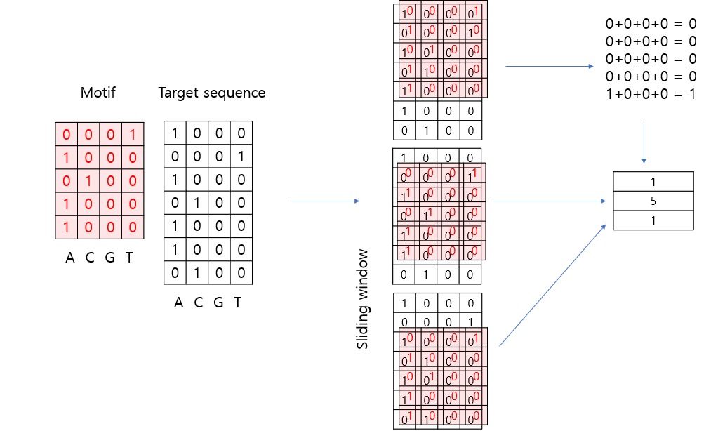
If there is a ‘5’ in the length-3 array as shown above, it indicates that the target sequence contains a sequence matching the motif.
To search for the presence of the PWM motif in the sequence “ATACAA,” a sliding window of length 5 can be used to divide the sequence into two sub-sequences: “ATACA” and “TACAA.”
pwm_arr = np.array(list(pwm.values())).transpose()
print(pwm_arr.shape)

print(onehot_encode.shape)
print(onehot_encode[0:5,].shape)
print(onehot_encode[1:6,].shape)

s1 = np.multiply(onehot_encode[0:5,], pwm_arr)
s2 = np.multiply(onehot_encode[1:6,], pwm_arr)
print(s1)
print(s2)

print(np.sum(s1, axis=1))
print(np.prod(np.sum(s1, axis=1)))

print(np.log(np.prod(np.sum(s1, axis=1)))) #s1 score
print(np.log(np.prod(np.sum(s2, axis=1)))) #s2 score
(5, 4)
(6, 4)
(5, 4)
(5, 4)
[[0.1 0. 0. 0. ]
[0. 0. 0. 0.1]
[0.1 0. 0. 0. ]
[0. 0.1 0. 0. ]
[0.7 0. 0. 0. ]]
[[0. 0. 0. 0.7]
[0.7 0. 0. 0. ]
[0. 0.7 0. 0. ]
[0.5 0. 0. 0. ]
[0.7 0. 0. 0. ]]
[0.1 0.1 0.1 0.1 0.7]
7.000000000000002e-05
-9.567015315914915
-2.119846956314875
Generate 1,000 simulated positive sequences by embedding a motif in the middle of the sequences, and 1,000 negative sequences with random DNA sequences.
import numpy as np
seq_length = 20
num_sample = 1000
#motif CCGGAA
motif_pwm = np.array([[10.41, 22.86, 1.92, 1.55, 98.60, 86.66],
            [68.20, 65.25, 0.50, 0.35, 0.25, 2.57],
            [17.27, 8.30, 94.77, 97.32, 0.87, 0.00],
            [4.13, 3.59, 2.81, 0.78, 0.28, 10.77]])
pwm = np.hstack([np.ones((4, 7)), motif_pwm, np.ones((4, 7))])
pos = np.array([np.random.choice( ['A', 'C', 'G', 'T'], num_sample,
                                  p=pwm[:,i]/sum(pwm[:,i])) for i in range(seq_length)]).transpose()
neg = np.array([np.random.choice( ['A', 'C', 'G', 'T'], num_sample,
                                  p=np.array([1,1,1,1])/4) for i in range(seq_length)]).transpose()

print(pos.shape)
display([''.join(x) for x in pos[1:5,]])
print()
display([''.join(x) for x in neg[1:5,]])
(1000, 20)
['GGATTAAACGGAAACTATTT',
 'AAGACTGCCGGATGGGCTCG',
 'CCCGAAGGCGGAAACAATCT',
 'ATGGAAGCGGGAAATATTCT']
['CTACCCTTACTCGCAGGGAA',
'ACTCACTAATTGGATTGAGA',
'AGGTACCTCGCGGCATCTGG',
'GGTATCTACGTGAAGAAGGG']base_dict = {'A':0, 'C':1, 'G':2, 'T':3}
# response variable for pos
onehot_encode_pos = np.zeros((num_sample, seq_length, 4))
onehot_encode_pos_label = np.zeros((num_sample, 2), dtype=int)
onehot_encode_pos_label[:,0] = 1
# print(onehot_encode_pos_label)
# response variable for pos
onehot_encode_neg = np.zeros((num_sample, seq_length, 4))
onehot_encode_neg_label = np.zeros((num_sample, 2), dtype=int)
onehot_encode_neg_label[:,1] = 1
# print(onehot_encode_neg_label)
# convert sequence to onehot
for i in range(num_sample):
for j in range(seq_length):
onehot_encode_pos[i,j,base_dict[pos[i,j]]] = 1
onehot_encode_neg[i,j,base_dict[neg[i,j]]] = 1
# concatenation
X = np.vstack((onehot_encode_pos, onehot_encode_neg))
y = np.vstack((onehot_encode_pos_label, onehot_encode_neg_label))
print(X.shape, y.shape)
# (2000, 20, 4) (2000, 2)(2000, 20, 4) (2000, 2)import torch
from torch.utils.data import TensorDataset, DataLoader
from sklearn.model_selection import train_test_split
# 데이터를 훈련 세트와 테스트 세트로 나눔
X_train, X_test, y_train, y_test = train_test_split(X, y, test_size=0.2, random_state=125)
print(X_train.shape, y_train.shape)
# NumPy 배열을 PyTorch 텐서로 변환
X_train = torch.tensor(X_train, dtype=torch.float32).transpose(1,2)
X_test = torch.tensor(X_test, dtype=torch.float32).transpose(1,2)
y_train = torch.tensor(y_train, dtype=torch.float32)
y_test = torch.tensor(y_test, dtype=torch.float32)
print(y_test.dtype)
# DataLoader 설정
train_dataset = TensorDataset(X_train, y_train)
train_loader = DataLoader(train_dataset, batch_size=64, shuffle=True)
print(train_loader.dataset.tensors[0].shape)
print(train_loader.dataset.tensors[1].shape)
test_dataset = TensorDataset(X_test, y_test)
test_loader = DataLoader(test_dataset, batch_size=64, shuffle=False)(1600, 20, 4) (1600, 2)
torch.float32
torch.Size([1600, 4, 20])
torch.Size([1600, 2])import torch
X_torch = torch.tensor(X_train, dtype=torch.float32)
print(X_torch.shape)torch.Size([1600, 4, 20])/tmp/ipykernel_2688/3124571761.py:3: UserWarning: To copy construct from a tensor, it is recommended to use sourceTensor.clone().detach() or sourceTensor.clone().detach().requires_grad_(True), rather than torch.tensor(sourceTensor).
X_torch = torch.tensor(X_train, dtype=torch.float32)import torch.nn as nn
import torch.optim as optim
import torch
import torch.nn as nn
import torch.optim as optim
class DNA_CNN(nn.Module):
def __init__(self):
super(DNA_CNN, self).__init__()
self.conv1 = nn.Conv1d(in_channels=4, out_channels=16, kernel_size=3, padding=1)
self.relu = nn.ReLU()
self.maxpool = nn.MaxPool1d(kernel_size=2)
self.flatten = nn.Flatten()
self.fc1 = nn.Linear(160, 64) # Adjust the input features according to your pooling and conv1d output
self.fc2 = nn.Linear(64, 2) # Adjust according to your problem's needs (e.g., number of classes)
#self.softmax = nn.Softmax(dim=1)
def forward(self, x):
x = self.conv1(x)
x = self.relu(x)
x = self.maxpool(x)
x = self.flatten(x)
x = self.fc1(x)
x = self.fc2(x)
#x = self.softmax(x)
return x
model = DNA_CNN()
if torch.cuda.is_available():
model.cuda()
# Loss and optimizer
criterion = nn.CrossEntropyLoss()
optimizer = optim.Adam(model.parameters(), lr=0.001)
from torchsummary import summary
summary(model, input_size=(4, 20)) # (Channels, Length)----------------------------------------------------------------
Layer (type) Output Shape Param #
================================================================
Conv1d-1 [-1, 16, 20] 208
ReLU-2 [-1, 16, 20] 0
MaxPool1d-3 [-1, 16, 10] 0
Flatten-4 [-1, 160] 0
Linear-5 [-1, 64] 10,304
Linear-6 [-1, 2] 130
================================================================
Total params: 10,642
Trainable params: 10,642
Non-trainable params: 0
----------------------------------------------------------------
Input size (MB): 0.00
Forward/backward pass size (MB): 0.01
Params size (MB): 0.04
Estimated Total Size (MB): 0.05
----------------------------------------------------------------# 훈련 루프
num_epochs = 20
for epoch in range(num_epochs):
for inputs, labels in train_loader:
if torch.cuda.is_available():
inputs, labels = inputs.cuda(), labels.cuda()
# Forward pass
outputs = model(inputs)
loss = criterion(outputs, labels)
# Backward and optimize
optimizer.zero_grad()
loss.backward()
optimizer.step()
print(f'Epoch [{epoch+1}/{num_epochs}], Loss: {loss.item():.4f}')
Epoch [1/20], Loss: 0.5050
Epoch [2/20], Loss: 0.2472
Epoch [3/20], Loss: 0.1437
Epoch [4/20], Loss: 0.0821
Epoch [5/20], Loss: 0.0966
Epoch [6/20], Loss: 0.0719
Epoch [7/20], Loss: 0.0729
Epoch [8/20], Loss: 0.0387
Epoch [9/20], Loss: 0.1018
Epoch [10/20], Loss: 0.1520
Epoch [11/20], Loss: 0.0712
Epoch [12/20], Loss: 0.0277
Epoch [13/20], Loss: 0.0272
Epoch [14/20], Loss: 0.0318
Epoch [15/20], Loss: 0.0215
Epoch [16/20], Loss: 0.0464
Epoch [17/20], Loss: 0.0975
Epoch [18/20], Loss: 0.0566
Epoch [19/20], Loss: 0.0191
Epoch [20/20], Loss: 0.0516# 모델 평가
model.eval()
with torch.no_grad():
correct = 0
total = 0
for inputs, labels in test_loader:
if torch.cuda.is_available():
inputs, labels = inputs.cuda(), labels.cuda()
outputs = model(inputs)
#print(outputs.data)
_, predicted = torch.max(outputs.data, 1)
#print(predicted)
total += labels.size(0)
labels_max = torch.max(labels, 1)[1]
#print(labels_max)
correct += (predicted == labels_max).sum().item()
print(f'Accuracy of the model on the test images: {100 * correct / total} %')Accuracy of the model on the test images: 98.5 %import matplotlib.pyplot as plt
# 데이터 저장을 위한 리스트 초기화
train_losses = []
val_accuracies = []
num_epochs = 200
for epoch in range(num_epochs):
model.train()
running_loss = 0.0
for inputs, labels in train_loader:
if torch.cuda.is_available():
inputs, labels = inputs.cuda(), labels.cuda()
# Forward pass
outputs = model(inputs)
loss = criterion(outputs, labels)
# Backward and optimize
optimizer.zero_grad()
loss.backward()
optimizer.step()
running_loss += loss.item() * inputs.size(0)
epoch_loss = running_loss / len(train_loader.dataset)
train_losses.append(epoch_loss)
# 모델 평가
model.eval()
correct = 0
total = 0
with torch.no_grad():
for inputs, labels in test_loader:
if torch.cuda.is_available():
inputs, labels = inputs.cuda(), labels.cuda()
outputs = model(inputs)
_, predicted = torch.max(outputs.data, 1)
total += labels.size(0)
labels_max = torch.max(labels, 1)[1]
correct += (predicted == labels_max).sum().item()
epoch_accuracy = 100 * correct / total
val_accuracies.append(epoch_accuracy)
print(f'Epoch [{epoch+1}/{num_epochs}], Loss: {epoch_loss:.4f}, Accuracy: {epoch_accuracy:.2f}%')
# 그래프 그리기
plt.figure(figsize=(12, 5))
plt.subplot(1, 2, 1)
plt.plot(train_losses, label='Training Loss')
plt.title('Training Loss')
plt.xlabel('Epoch')
plt.ylabel('Loss')
plt.legend()
plt.subplot(1, 2, 2)
plt.plot(val_accuracies, label='Validation Accuracy')
plt.title('Validation Accuracy')
plt.xlabel('Epoch')
plt.ylabel('Accuracy (%)')
plt.legend()
plt.show()NameError: name 'model' is not defined