from google.colab import drive
import os

drive.mount('/content/drive')
os.chdir('drive/MyDrive/2024-cnu-lecture')4 Data handling
!pwd4.0.1 [User]
I want to learn “2. Data Handling and Analysis”. can you explain me a brief explanation and examples?
4.0.2 [ChatGPT]
Sure! Data handling and analysis are essential skills in Python, especially for tasks like manipulating datasets, performing statistical analyses, and creating visualizations. We’ll focus on the key libraries used for these purposes: NumPy, Pandas, and Matplotlib/Seaborn.
4.0.3 1. NumPy
NumPy is a powerful library for numerical operations and handling arrays.
4.0.3.1 Basics of NumPy
Installation:
!pip install numpyimport numpy as np
# Creating a 1D array
arr1 = np.array([1, 2, 3, 4, 5])
# Creating a 2D array
arr2 = np.array([[1, 2, 3], [4, 5, 6]])
print(arr1)
print(arr2)
# Element-wise operations
arr3 = arr1 * 2
print(arr3)
# Mathematical functions
print(np.sqrt(arr1))[1 2 3 4 5]
[[1 2 3]
[4 5 6]]
[ 2 4 6 8 10]
[1. 1.41421356 1.73205081 2. 2.23606798]4.0.3.2 Numpy 자료구조 ndarray
행렬이나 다차원 배열 처리용 파이썬 라이브러리
같은 타입의 데이터만 허용
리스트에 비해 20배 이상 빠른 속도
numpy 배열의 가시화는 일반적으로 우리가 사용하는 방식과 다름
일반적으로 우리는 차원을 높여가며 그림을 그릴 경우 아래와 같음
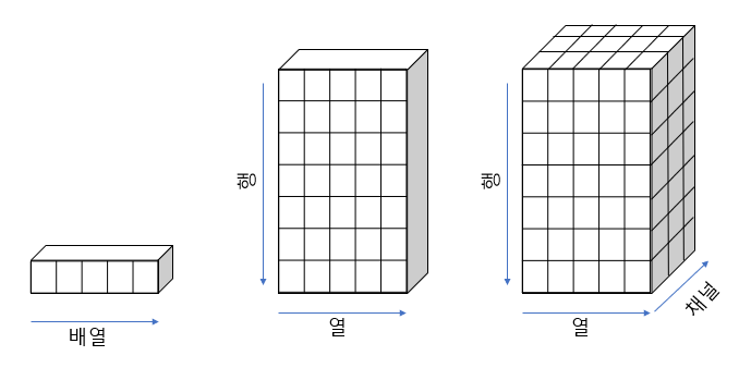
- 그런데 numpy에서 차원의 추가는 shape의 앞쪽에 새로운 차원이 추가가 되는 형식
- 그림으로 그릴 경우 아래와 같이 axis 0, 1, 2 순서로 해석될 수 있음
import numpy as np

display(np.ones(4))
display(np.ones((3, 4)))
display(np.ones((2, 3, 4)))
array([1., 1., 1., 1.])array([[1., 1., 1., 1.],
[1., 1., 1., 1.],
[1., 1., 1., 1.]])array([[[1., 1., 1., 1.],
[1., 1., 1., 1.],
[1., 1., 1., 1.]],
[[1., 1., 1., 1.],
[1., 1., 1., 1.],
[1., 1., 1., 1.]]])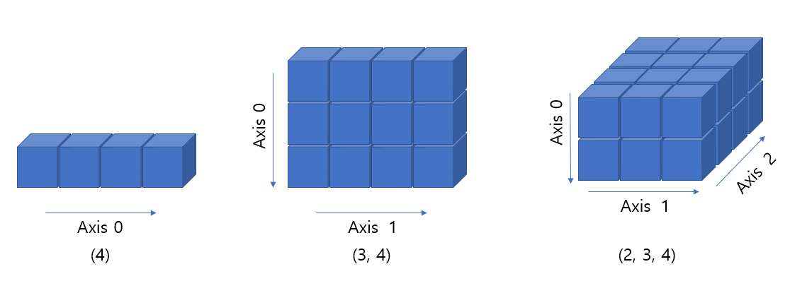
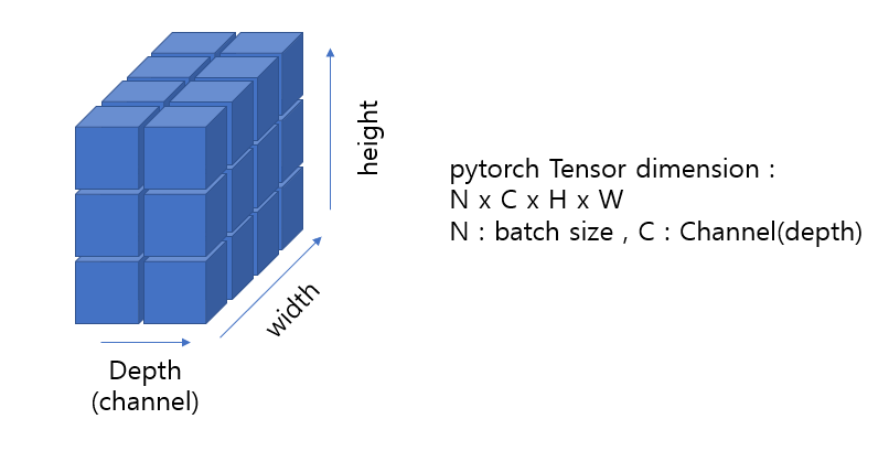
- 위와 같이 표현되는 것이 맞으나 기존 우리가 알고 있는 가시화 방식과 차이가 있어 혼란 가능
- 또한, 아래 pytorch의 tensor dimension 표현법은 또 다른 방식임
- 따라서 각 dimension의 axis를 구분하는 것 보다는 depth (channel), width, height를 명확하게 구분하는 것이 중요하고 상황에 따라 다르게 가시화 할 수 있도록 훈련 필요
- numpy 객체 만들기
import numpy as np

arr = [1, 2, 3]
print(arr)
print(type(arr))

a = np.array([1,2,3])
print(a)
print(a.dtype)
print(a.shape)
print(type(a))
[1, 2, 3]
<class 'list'>
[1 2 3]
int64
(3,)
<class 'numpy.ndarray'>arr2 = np.array([[1,2,3], [4,5,6]])
print(arr2)
print(type(arr2))
print(arr2.shape)
print(arr2.dtype)[[1 2 3]
[4 5 6]]
<class 'numpy.ndarray'>
(2, 3)
int64- numpy 자료형
- 부호가 있는 정수 int(8, 16, 32, 64)
- 부호가 없는 정수 uint(8 ,16, 32, 54)
- 실수 float(16, 32, 64, 128)
- 복소수 complex(64, 128, 256)
- 불리언 bool
- 문자열 string_
- 파이썬 오프젝트 object
- 유니코드 unicode_
- np.zeros(), np.ones(), np.arange()
- 행렬 연산 지원
a = np.arange(1, 10).reshape(3,3) # [1, 10)
print(a)
a = np.ones((3,4), dtype=np.int16)
b = np.ones((3,4), dtype=np.int16)
print(a)
print(b)
print(a+b)
print(a-b)
[[1 2 3]
[4 5 6]
[7 8 9]]
[[1 1 1 1]
[1 1 1 1]
[1 1 1 1]]
[[1 1 1 1]
[1 1 1 1]
[1 1 1 1]]
[[2 2 2 2]
[2 2 2 2]
[2 2 2 2]]
[[0 0 0 0]
[0 0 0 0]
[0 0 0 0]]- numpy 함수
- np.sqrt()
- np.log()
- np.square()
- np.log()
- np.ceil()
- np.floor()
- np.isnan()
- np.sum()
- np.mean()
- np.std()
- np.min()
dir(np)4.0.4 2. Pandas
Pandas is a powerful library for data manipulation and analysis. It provides data structures like DataFrame, which is similar to tables in databases or spreadsheets.
4.0.4.1 Installation
pip install pandas- Pandas의 Series는 1차원, DataFrame은 2차원 데이터를 다루는 자료구조
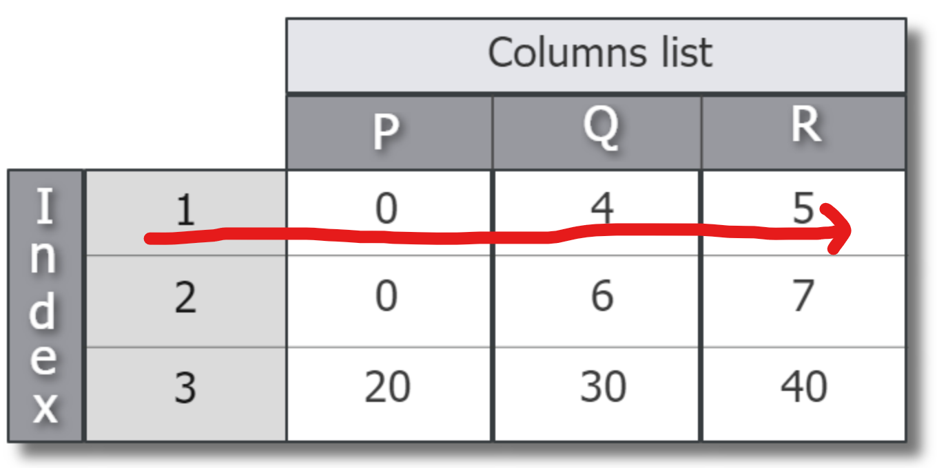
- DataFrames are the primary data structure in pandas, representing tabular data with rows and columns.
- index, column, values 로 이루어짐
- 리스트와 딕셔너리로부터 생성 가능
- 숫자형, 문자형, 범주형 등의 다양한 데이터 입력 가능
from pandas import Series, DataFramegenes = Series([0.1, 0.2, 1.4, 0.6, 1.1])
print(genes)0 0.1
1 0.2
2 1.4
3 0.6
4 1.1
dtype: float64genes = Series([0.1, 0.2, 1.4, 0.6, 1.1], index=['A', 'B', 'C', 'D', 'E'])
print(genes)A 0.1
B 0.2
C 1.4
D 0.6
E 1.1
dtype: float644.0.4.2 Make a DataFrame
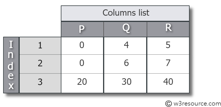
- Create from a list
import pandas as pd

df = pd.DataFrame([[0, 4, 5], [0, 6, 7], [20, 30, 40]],
                  index=[1, 2, 3], columns=['P', 'Q', 'R'])

print(df)
P Q R
1 0 4 5
2 0 6 7
3 20 30 40- Create dataframe from a dictionary

import pandas as pd

data = {
    'Name': ['Alice', 'Bob', 'Charlie'],
    'Age': [25, 30, 35],
    'Height': [5.5, 6.0, 5.8]
}

df = pd.DataFrame(data)
print(df)
Name Age Height
0 Alice 25 5.5
1 Bob 30 6.0
2 Charlie 35 5.8- Create from a list of dictionary
data = [
{'Name': 'Alice', 'Age': 25, 'Height': 5.5},
{'Name': 'Bob', 'Age': 30, 'Height': 6.0},
{'Name': 'Charlie', 'Age': 35, 'Height': 5.8}
]
df = pd.DataFrame(data)
print(df) Name Age Height
0 Alice 25 5.5
1 Bob 30 6.0
2 Charlie 35 5.8- Create from Series
genes = {'A': [0.5, 0.1, 0.3],
'B': [0.8, 0.9, 0.4]}
print(genes)
genes_df = DataFrame(genes)
print(genes_df)
print(genes_df['A'])
print(type(genes_df['A']))
genes_df = DataFrame(genes, columns=['B', 'A'], index=['day1', 'day2', 'day3'])
print(genes_df){'A': [0.5, 0.1, 0.3], 'B': [0.8, 0.9, 0.4]}
A B
0 0.5 0.8
1 0.1 0.9
2 0.3 0.4
0 0.5
1 0.1
2 0.3
Name: A, dtype: float64
<class 'pandas.core.series.Series'>
B A
day1 0.8 0.5
day2 0.9 0.1
day3 0.4 0.34.0.4.3 Dataframe operations
data = [
{'Name': 'Alice', 'Age': 25, 'Height': 5.5},
{'Name': 'Bob', 'Age': 30, 'Height': 6.0},
{'Name': 'Charlie', 'Age': 35, 'Height': 5.8}
]
df = pd.DataFrame(data)
print(df)
      Name  Age  Height
0    Alice   25     5.5
1      Bob   30     6.0
2 Charlie 35 5.8# Selecting columns
ages = df['Age']
print(ages)
# Filtering rows
adults = df[df['Age'] > 18]
print(adults)
# Adding a new column
df['Weight'] = [65, 70, 75]
print(df)
# Grouping and Aggregating
grouped = df.groupby('Name').mean()
print(grouped)0 25
1 30
2 35
Name: Age, dtype: int64
Name Age Height
0 Alice 25 5.5
1 Bob 30 6.0
2 Charlie 35 5.8
Name Age Height Weight
0 Alice 25 5.5 65
1 Bob 30 6.0 70
2 Charlie 35 5.8 75
Age Height Weight
Name
Alice 25.0 5.5 65.0
Bob 30.0 6.0 70.0
Charlie 35.0 5.8 75.0- 인덱스 자동 정렬, 행렬 연산
genes1 = Series([0.1, 0.2, 1.4, 0.6, 1.1], index=['A', 'B', 'C', 'D', 'E'])
genes2 = Series([0.1, 0.2, 1.4, 0.6, 1.1], index=['B', 'C', 'D', 'E', 'A'])
genes1 + genes2A 1.2
B 0.3
C 1.6
D 2.0
E 1.7
dtype: float64print(genes2.sort_values())
print(genes2.sort_index())B 0.1
C 0.2
E 0.6
A 1.1
D 1.4
dtype: float64
A 1.1
B 0.1
C 0.2
D 1.4
E 0.6
dtype: float64genes = {'A': [0.5, 0.1, 0.3],
'B': [0.8, 0.9, 0.4]}
genes_df = DataFrame(genes, columns=['B', 'A'], index=['day1', 'day2', 'day3'])
print(genes)
print(genes_df){'A': [0.5, 0.1, 0.3], 'B': [0.8, 0.9, 0.4]}
B A
day1 0.8 0.5
day2 0.9 0.1
day3 0.4 0.3print(genes_df['A'])
print(genes_df.loc['day1'])
print(genes_df.index)
print(list(genes_df.columns))day1 0.5
day2 0.1
day3 0.3
Name: A, dtype: float64
B 0.8
A 0.5
Name: day1, dtype: float64
Index(['day1', 'day2', 'day3'], dtype='object')
['B', 'A']4.0.5 3. Matplotlib/Seaborn
Matplotlib is a plotting library for creating static, animated, and interactive visualizations. Seaborn is built on top of Matplotlib and provides a high-level interface for drawing attractive statistical graphics.
Installation:
pip install matplotlib seabornimport matplotlib.pyplot as plt
# Line plot
plt.plot([1, 2, 3, 4], [1, 4, 9, 16])
plt.xlabel('X-axis')
plt.ylabel('Y-axis')
plt.title('Line Plot')
plt.show()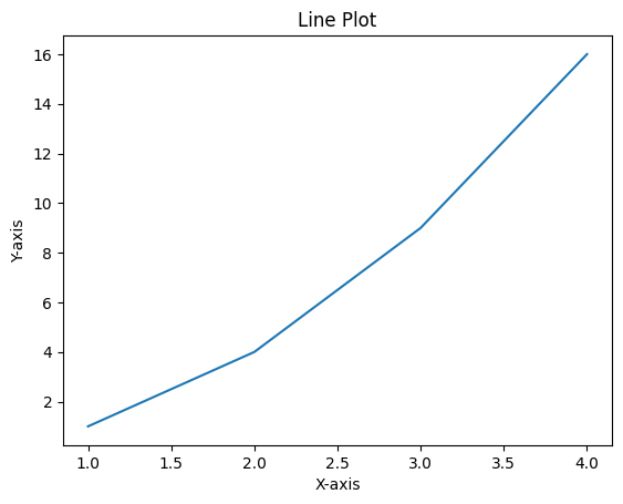
import matplotlib.pyplot as plt
import seaborn as sns
data = [
    {'Name': 'Alice', 'Age': 25, 'Height': 5.5},
    {'Name': 'Bob', 'Age': 30, 'Height': 6.0},
    {'Name': 'Charlie', 'Age': 35, 'Height': 5.8}
]

df = pd.DataFrame(data)
print(df)
# Scatter plot with Seaborn
sns.scatterplot(x='Age', y='Height', data=df)
plt.title('Age vs Height')
plt.show() Name Age Height
0 Alice 25 5.5
1 Bob 30 6.0
2 Charlie 35 5.8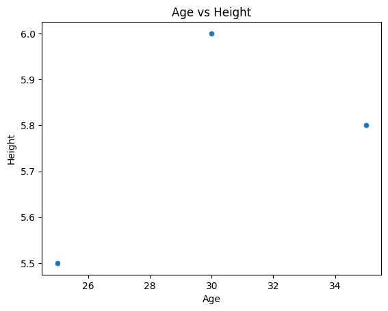
dir(sns)4.0.6 Example: Analyzing and Visualizing DNA Sequence Data
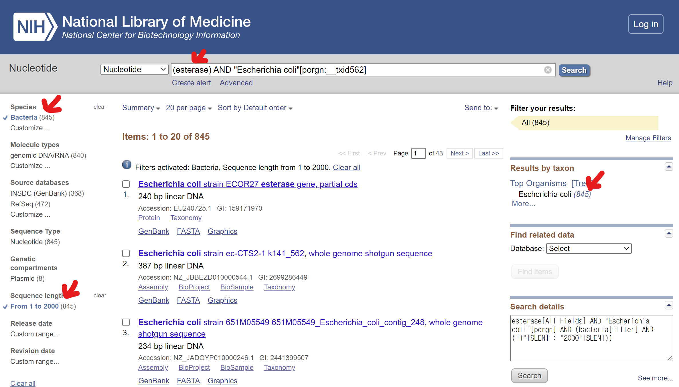
4.0.6.1 [User]
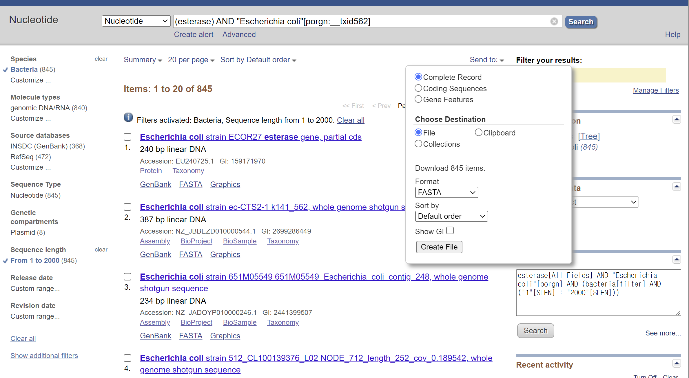
I have downloaded a fasta file containing 800 esterase nucleotide sequences. the file is saved at “data/esterase.fa”. can you provide a python code that can read the sequences and compute their length and GC contents ratio?
4.0.6.2 [ChatGPT]
Certainly! To read a FASTA file containing 800 esterase nucleotide sequences and compute their lengths and GC content ratios, you can use the Biopython library. Here is a Python script that accomplishes this:
Installation
First, make sure you have Biopython installed:
pip install biopythonfrom Bio import SeqIO
from Bio.SeqUtils import gc_fraction
# Function to compute sequence length and GC content
def compute_sequence_stats(seq):
length = len(seq)
gc_content = gc_fraction(seq) * 100 # Convert to percentage
return length, gc_content
# Read the FASTA file and process each sequence
def process_fasta_file(file_path):
records = SeqIO.parse(file_path, "fasta")
esterase_stats = []
for record in records:
length, gc_content = compute_sequence_stats(record.seq)
esterase_stats.append({
"ID": record.id,
"Length": length,
"GC_Content": gc_content
})
return esterase_stats
# Example usage
fasta_file = 'data/esterases.fasta' # Replace with your FASTA file path
esterase_stats = process_fasta_file(fasta_file)
# Print the results
for esterase in esterase_stats:
print(f"ID: {esterase['ID']}, Length: {esterase['Length']} bp, GC Content: {esterase['GC_Content']:.2f}%")4.0.6.3 [User]
I want to store the result above in a file with json csv format. Than I need a code to read the file and convert the data in a DataFrame format.
4.0.6.4 [ChatGPT]
Sure! Let’s modify the script to store the results in both JSON and CSV formats. Then, we’ll write a separate script to read these files and convert the data into a Pandas DataFrame.
import json
import csv
from Bio import SeqIO
from Bio.SeqUtils import gc_fraction

# Function to compute sequence length and GC content
def compute_sequence_stats(seq):
    length = len(seq)
    gc_content = gc_fraction(seq) * 100  # Convert to percentage
    return length, gc_content

# Read the FASTA file and process each sequence
def process_fasta_file(file_path):
    records = SeqIO.parse(file_path, "fasta")
    esterase_stats = []

    for record in records:
        length, gc_content = compute_sequence_stats(record.seq)
        esterase_stats.append({
            "ID": record.id,
            "Length": length,
            "GC_Content": gc_content
        })

    return esterase_stats

# Save results to JSON and CSV
def save_results(esterase_stats, json_file, csv_file):
    # Save to JSON
    with open(json_file, 'w') as jf:
        json.dump(esterase_stats, jf, indent=4)

    # Save to CSV
    with open(csv_file, 'w', newline='') as cf:
        writer = csv.DictWriter(cf, fieldnames=['ID', 'Length', 'GC_Content'])
        writer.writeheader()
        for esterase in esterase_stats:
            writer.writerow(esterase)

# Example usage
fasta_file = 'data/esterases.fasta'  # Replace with your FASTA file path
json_file = 'data/esterase_stats.json'
csv_file = 'data/esterase_stats.csv'

esterase_stats = process_fasta_file(fasta_file)
save_results(esterase_stats, json_file, csv_file)

print(f"Results saved to {json_file} and {csv_file}")
Results saved to data/esterase_stats.json and data/esterase_stats.csvimport pandas as pd
import json
# Load data from JSON file
with open('data/esterase_stats.json', 'r') as jf:
esterase_stats_json = json.load(jf)
# Convert to DataFrame
df_json = pd.DataFrame(esterase_stats_json)
print("DataFrame from JSON file:")
print(df_json.head())
# Load data from CSV file
df_csv = pd.read_csv('data/esterase_stats.csv')
print("DataFrame from CSV file:")
print(df_csv.head())4.0.6.5 [User]
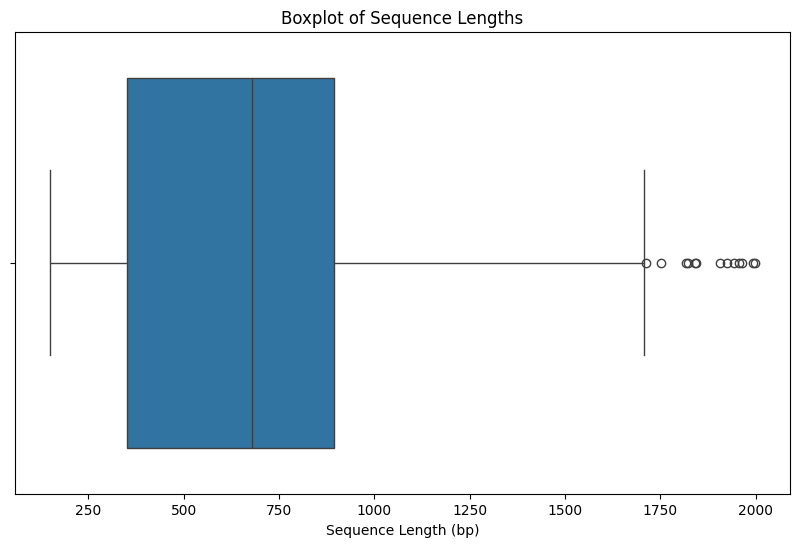
I want a python code that display the statistics of the GC distribution and boxplot of the length.
4.0.6.6 [ChatGPT]
Sure! Let’s create a Python script that reads the data from the previously saved JSON or CSV file, computes statistics for the GC content distribution, and generates a boxplot for the sequence lengths using Pandas and Matplotlib.
import pandas as pd
import matplotlib.pyplot as plt
import seaborn as sns

# Load data from CSV file
df = pd.read_csv('data/esterase_stats.csv')

# Compute statistics for GC content distribution
gc_stats = df['GC_Content'].describe()
print("GC Content Distribution Statistics:")
print(gc_stats)

# Generate a histogram for GC content distribution
plt.figure(figsize=(10, 6))
sns.histplot(df['GC_Content'], bins=30, kde=True)
plt.title('GC Content Distribution')
plt.xlabel('GC Content (%)')
plt.ylabel('Frequency')
plt.show()

# Generate a boxplot for sequence lengths
plt.figure(figsize=(10, 6))
sns.boxplot(x=df['Length'])
plt.title('Boxplot of Sequence Lengths')
plt.xlabel('Sequence Length (bp)')
plt.show()
GC Content Distribution Statistics:
count 355.000000
mean 51.362399
std 5.551809
min 29.739777
25% 50.052780
50% 51.901566
75% 54.322222
max 75.683891
Name: GC_Content, dtype: float64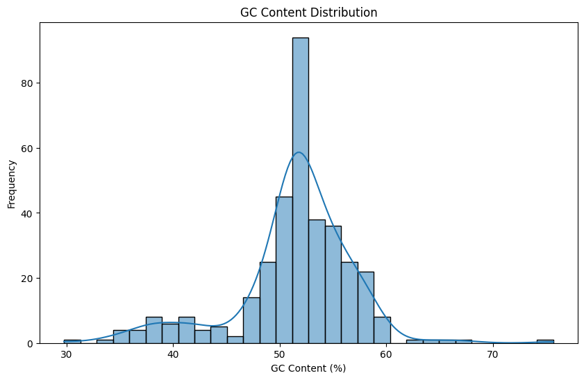
- Script
from Bio import SeqIO
from Bio.SeqUtils import gc_fraction

# Read a FASTA file
fasta_file = 'data/esterases.fasta'
results = SeqIO.parse(fasta_file, 'fasta')

for record in results:
    print(record.id)
    print(record.seq)
    print(gc_fraction(record.seq))

print(results)- Calculate
from Bio import SeqIO
from Bio.SeqUtils import gc_fraction

# Read a FASTA file
fasta_file = 'data/esterases.fasta'
results = SeqIO.parse(fasta_file, 'fasta')

for record in results:
    seq = record.seq
    length = len(seq)
    gc_content = gc_fraction(seq) * 100  # Convert to percentage
    print(f"ID: {record.id}, Length: {length} bp, GC Content: {gc_content:.2f}%")
- store in a list
from Bio import SeqIO
from Bio.SeqUtils import gc_fraction
import pandas as pd

# Read a FASTA file
fasta_file = 'data/esterases.fasta'
results = SeqIO.parse(fasta_file, 'fasta')
esterase_stats = []

for record in results:
    seq = record.seq
    length = len(seq)
    gc_content = gc_fraction(seq) * 100  # Convert to percentage
    esterase_stats.append({
        "ID": record.id,
        "Length": length,
        "GC_Content": gc_content
    })

print(esterase_stats)
pd.DataFrame(esterase_stats)- make a function
from Bio import SeqIO
from Bio.SeqUtils import gc_fraction
import pandas as pd

# Read a FASTA file
fasta_file = 'data/esterases.fasta'
results = SeqIO.parse(fasta_file, 'fasta')
esterase_stats = []

# Function to compute sequence length and GC content
def compute_sequence_stats(seq):
    length = len(seq)
    gc_content = gc_fraction(seq) * 100  # Convert to percentage
    return length, gc_content


for record in results:
    seq = record.seq
    length, gc_content = compute_sequence_stats(seq)
    esterase_stats.append({
        "ID": record.id,
        "Length": length,
        "GC_Content": gc_content
    })

print(esterase_stats)
pd.DataFrame(esterase_stats)